Syntouch BioTac Calibration and Closed-Loop Characterization
August 28, 2015
Overview
The BioTac by SynTouch is a biomemetic fingertip sensor that provides the ability to sense temperature, pressure, vibration, and point of contact similar to a human fingertip. Using its data it is possible to generate a force vector that can be used for real-time force sensing. This project has two purposes. The first is to formulate a calibration scheme for the BioTac’s sensors that can be used to convert its data output into a force in engineering units with particular attention paid to accounting for signal drift with temperature. The second is to characterize the system response of a closed-loop control system that is operating on the BioTac.
The BioTac
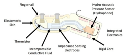
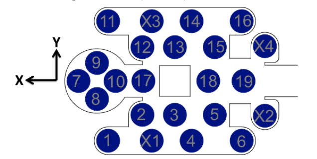
The BioTac consists of an elastomeric skin with a fluid-filled interior and an epoxy resin inner core. Embedded within the core are 19 sensing electrodes, four excitation electrodes, a thermistor, and a pressure sensor.
| Internal structure | Sensor layout |
|---|---|
 |
 |
The fluid within the skin is a conductive solution of sodium bromide. The sensing electrodes are used to measure its impedance, the thermistor is used to measure its temperature, and the pressure sensor measures the fluid’s current pressure and detects vibrations. All of this data is communicated from the BioTac over SPI.
Experimental Setup
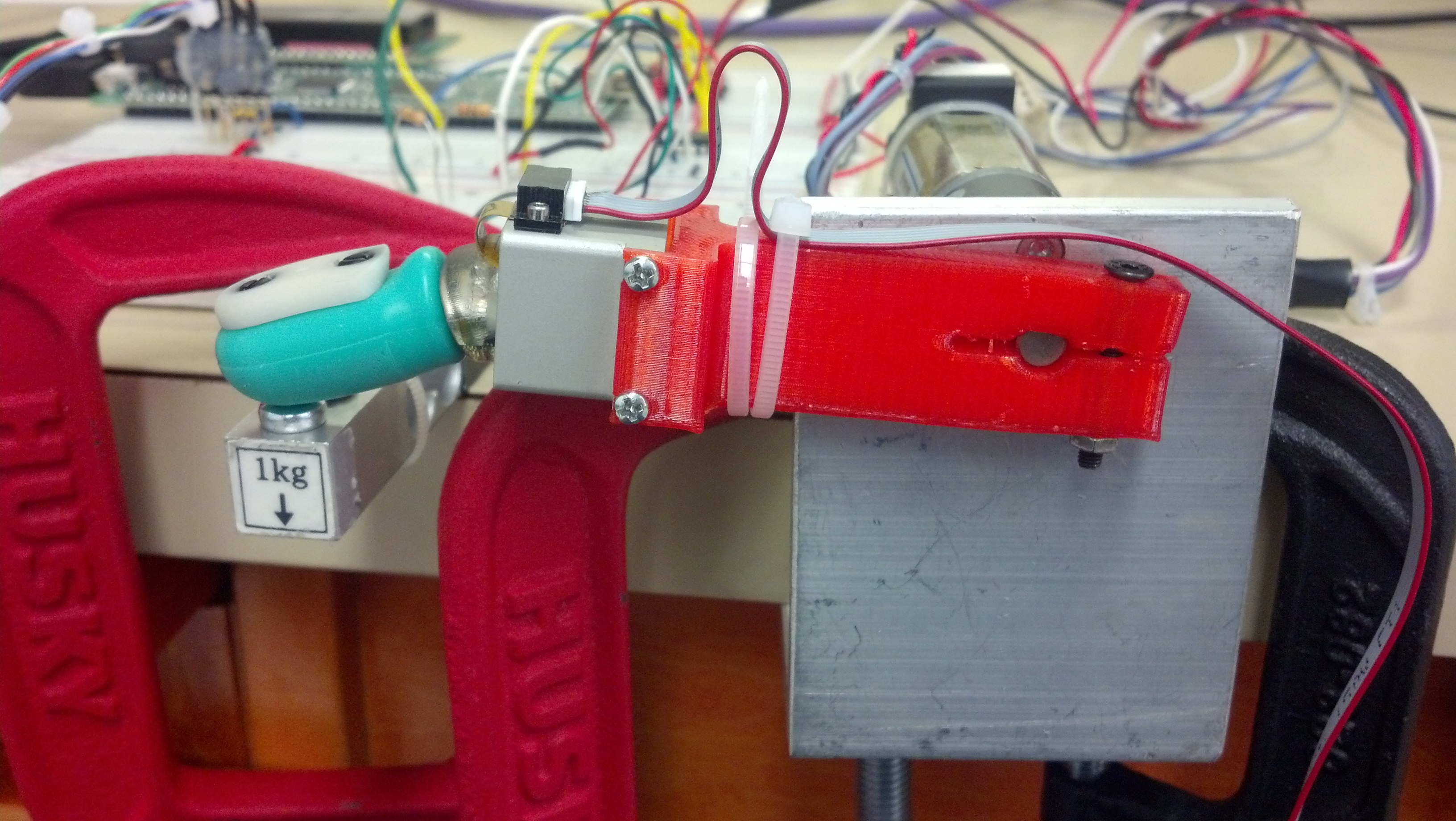
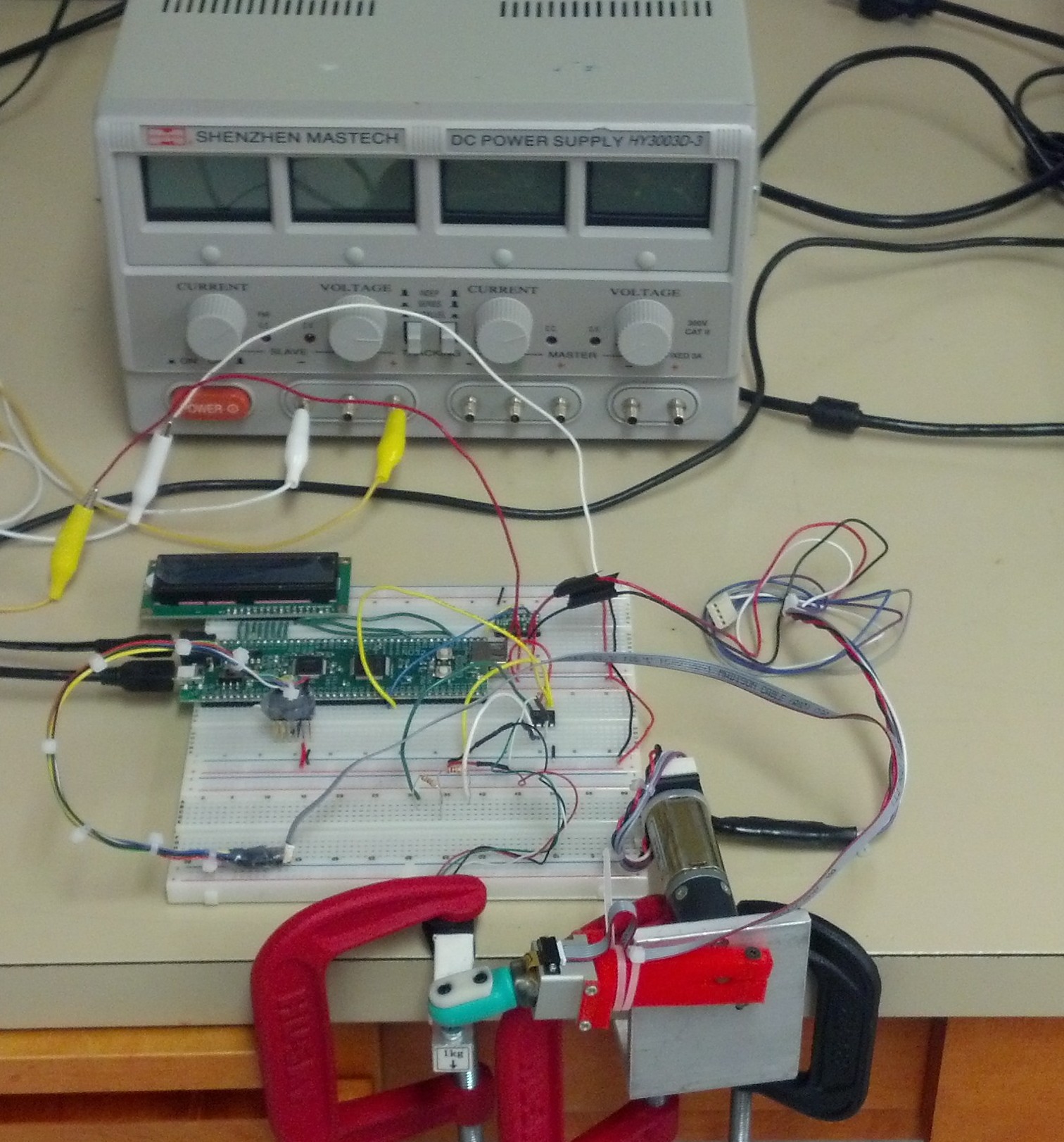
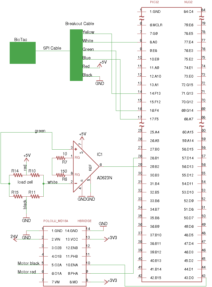
The setup consists of a brushless DC motor controlled through an H-bridge by a PIC32 to push the BioTac against a 1 kg load cell. The load cell is passed through an instrumentation amplifier, where the amplifier output is read by the PIC’s onboard ADC. The BioTac data is transmitted over SPI to the PIC. The PIC32 is mounted on a NU32 development board, which also houses a serial-to-USB converter. This serial connection is used to connect the PIC to a custom Linux GUI program and transmit BioTac, load cell, and other useful data via serial over USB for analysis, and also allows the program to control the PIC’s operation.
| Experimental Setup | Circuit Diagram |
|---|---|
 |
 |
 |
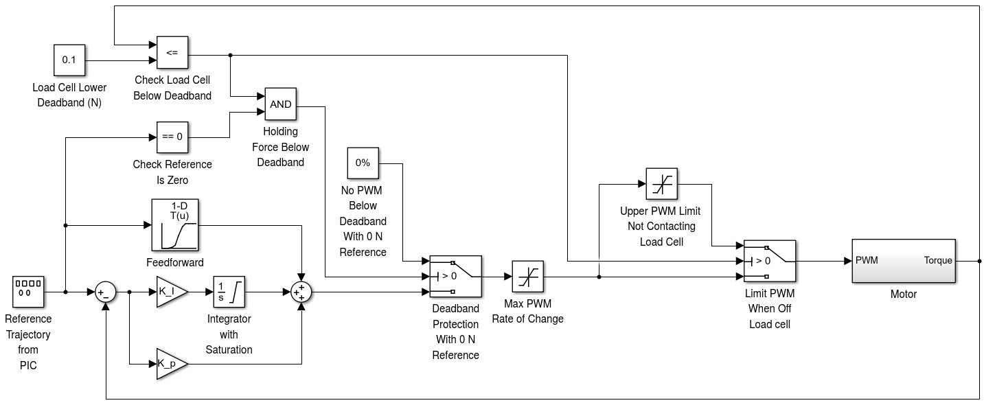
The closed-loop control system uses a combination of feedfoward and feedback control. The feedforward control consists of a simple linear model, determined through experimentation, that takes in a reference force value and generates a desired PWM signal. The feedback control consists of a PI controller that uses the load cell as its feedback. The controller also contains a few limiting features:
- A limit is placed on the maximum PWM if the BioTac is not contacting the load cell. This keeps the controller from slamming the BioTac.
- If the force exerted by the motor as measured by the load cell drops below a threshold (0.1N), the controller only lets the motor add force rather than move away from the load cell. In the particular situation that the reference force is 0 N and the load cell has a small amount of noise just above 0 N, the controller could cause the motor to continually drive the BioTac backwards. A small deadband is placed on the controller in this regim to keep the motor from backing off the load cell and gaining momentum.
- A limit is placed on the maximum amount of change of the PWM signal from iteration to iteration. Again, this protects the BioTac in case the system becomes unstable. This limit is purposely placed high and verified to not affect normal operation.
- Integrator anti-windup set to the value that would just allow the integral term alone to command 100% PWM duty cycle.
The load cell was calibrated by hanging weights of known mass, recording the raw ADC values, and generating a linear fit. The linear model is sufficient and accurate due to the very linear nature of the load cell.
Force Calibration
As previously mentioned, the skin of the BioTac is filled with a solution of sodium bromide. The sensing electrodes embedded within the core sense the fluid’s impedance by receiving a quick voltage pulse from the excitation electrodes and measuring the received voltage, which can be used to determine the impedance of the path through the fluid. This impedance changes as pressure is applied to the skin through contact, and it also changes with temperature. The change in impedance has already been used to determine a force vector and point of contact by Lin et al [1]. Lin’s method does so by removing the sensor from contact and taring the electrode values to provide a zero point from which to measure the change in electrodes as contact is made with the skin. The changes in the electrodes are then used in the following equation to produce the force vector.
\( \vec{F} = \langle S_x \sum_{i=1}^{19} e_i n_{x,i} , S_y \sum_{i=1}^{19} e_i n_{y,i} , S_z \sum_{i=1}^{19} e_i n_{z,i} \rangle \)
The S terms in the equation are scalars that are determined experimentally. The n values are normal vector components that correspond to each electrode. Although this method does generate a force vector, it does not attempt to continuously compensate for signal drift due to the current temperature. Instead it handles drift by periodically taring the electrodes to re-establish the zero points. This project’s aim was to characterize the signal drift with temperature and be able to continuously compensate for it in order to eliminate the need to periodically tare the electrodes.
Electrode Drift with Temperature
As the BioTac is operating, its internal electronics are generating heat, causing all parts of the BioTac to heat up. As the fluid temperature changes, its impedance also changes and causes the electrode values to drift as shown in this plot.
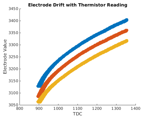
The x-axis represents the raw thermistor measurement, TDC, which corresponds to the current sensed temperature. The y-axis represents the raw electrode values. Each of these values arrives from the BioTac as a 12-bit value ranging from 0 to 4096. The temperature values shown range from 25.7 to 35.3 degrees Celsius.
Compensation of Drift
To compensate for this drift I tried using a non-linear least squares solving library, Ceres, to fit an exponential curve of the form
\( e_i=a_i(1-\mathrm{e}^{b_i\mathrm{TDC}+c_i})+d_i \)
where ei is an expected electrode value, TDC is the current TDC value from the BioTac, and the remaining terms (ai, bi, ci, and di) are all determined using the solver.
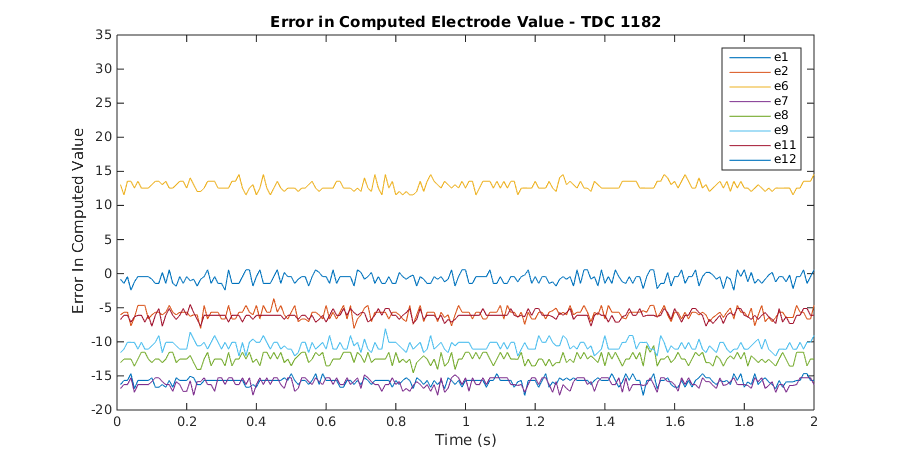
When I tried to fit the curves to the data, I found that it usually did not completely offset the electrodes. When I plotted the error between the expected electrode value and the actual recorded electrod value, I found that the fit was usually incorrect, sometimes by a significant amount. This even occurred at times when the temperature as measured by the thermistor is very similar as shown in these plots. These plots were generated by using BioTac data that was recorded while the BioTac was not in contact with anything to calculate an expected electrode value from TDC and compare it to the recorded electrode values to generate an error plot.
| Sample Errors 1 | Sample Errors 2 |
|---|---|
 |
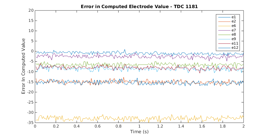 |
Notice that while some of the electrodes are at roughly the same value between the two plots, others are significantly different. This means that the temperature compensation model above is not sufficient to reliably calculate an accurate electrode value from temperature.
Force Calibration Results
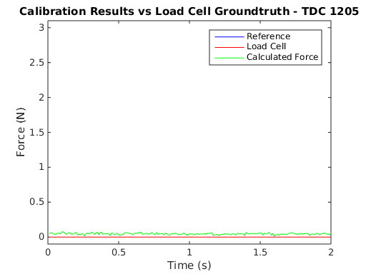
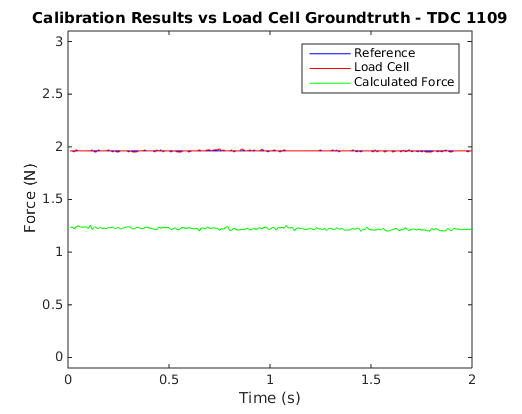
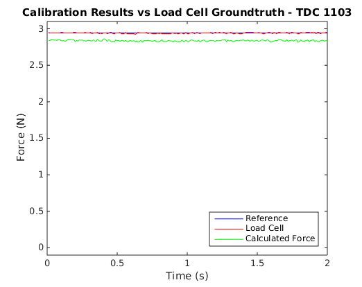
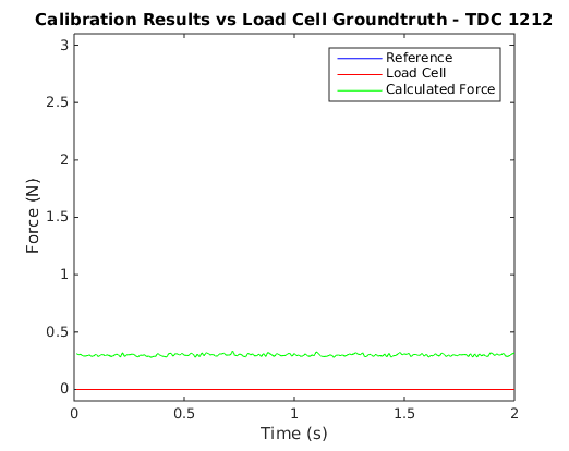
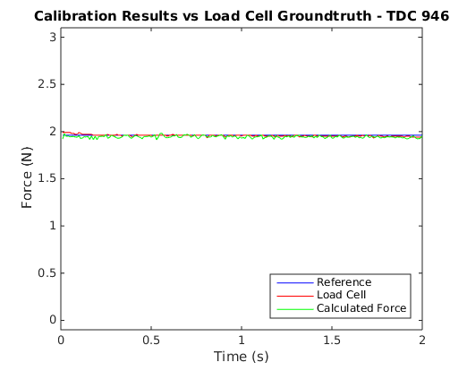
In an effort to see how the final force values work out given the electrode errors, I recorded some tests that used the brushed DC motor to press the BioTac against a 1 kg load cell and recorded the BioTac data and the load cell reading. I performed a large number of test runs over forces ranging from 0 N to 6 N and recorded all of their data to file. I then used my temperature compensation curves to offset the electrode values and used Ceres to solve for the S terms in the force equation above. Once these terms were solved, I used the calibration scheme to plot the function results with the target force for comparison. The following plots show some example outcomes.
| Results of 0N Test Runs (No Contact with BioTac) | Results of 2N Test Runs | Results of 3N Test Runs |
|---|---|---|
 |
 |
 |
 |
 |
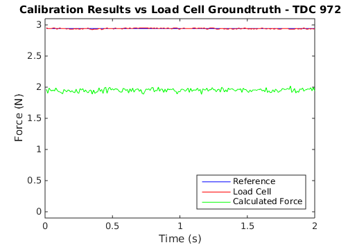 |
As can be seen, sometimes the results are quite accurate, but at other times the calculated value can differ by quite a bit.
Temperature Compensation Conclusions
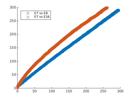
Modeling the temperature of the BioTac is much more complicated than being able to fit a curve as was being attempted. The main problem with fitting the data is the presence of temperature gradients within the fluid. There is only a single thermistor within the BioTac, so it is only able to sample the fluid temperature in its own vicinity. The following plots give an indication that gradients do exist within the fluid.
| Comparison of Electrodes 7, 8, and 16 | Comparison of Electrode 14, 17, and 18 |
|---|---|
 |
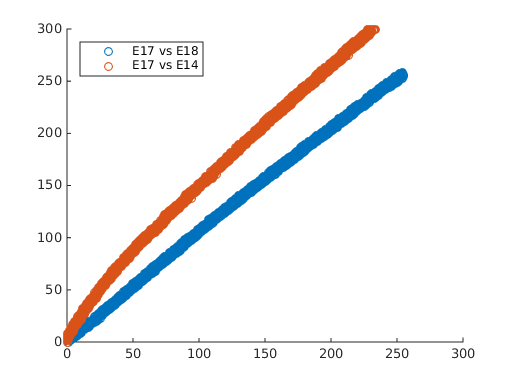 |
These plots were generated from the same data set that was used to create the plot above that shows how the electrodes change with TDC. The lines in these plots represent electrodes being compared against each other. As the fluid heats up, the electrodes increase in value as noted above. If the temperature of the fluid is the same throughout, the expectation is that all of the electrodes would change at the same rate or nearly the same rate. So if the electrodes are plotted against each other, they should exhibit a linear relationship as their values change. For these plots, the pairs of electrodes were chosen for spatial reasons. In the left-hand plot, electrodes 7 and 8 are located next to each other, while 7 and 16 are farther apart. And in the right-hand plot, electrodes 17 and 18 are close to each other while 17 and 14 are farther apart. As can be seen, the pairs 7/8 and 17/18 heat up at the same rate and show a linear relationship, whereas the other two pairs show a nonlinear relationship, which indicates the presence of local temperature gradients.
Additionally, the fluid, skin, and core each have different thermal properties and will heat at different rates, which further exacerbates the problem. And the overall problem is made particularly worse when the BioTac is contacting an object of different temperature. In summary, the temperature model of the BioTac is too complicated to be accounted by a single thermistor. While it may be useful for detecting contact with hot or cold objects or getting an idea of the temperature of the BioTac system, it cannot be used for a precision operation such as this one.
Closed-Loop System Characterization
Experiment
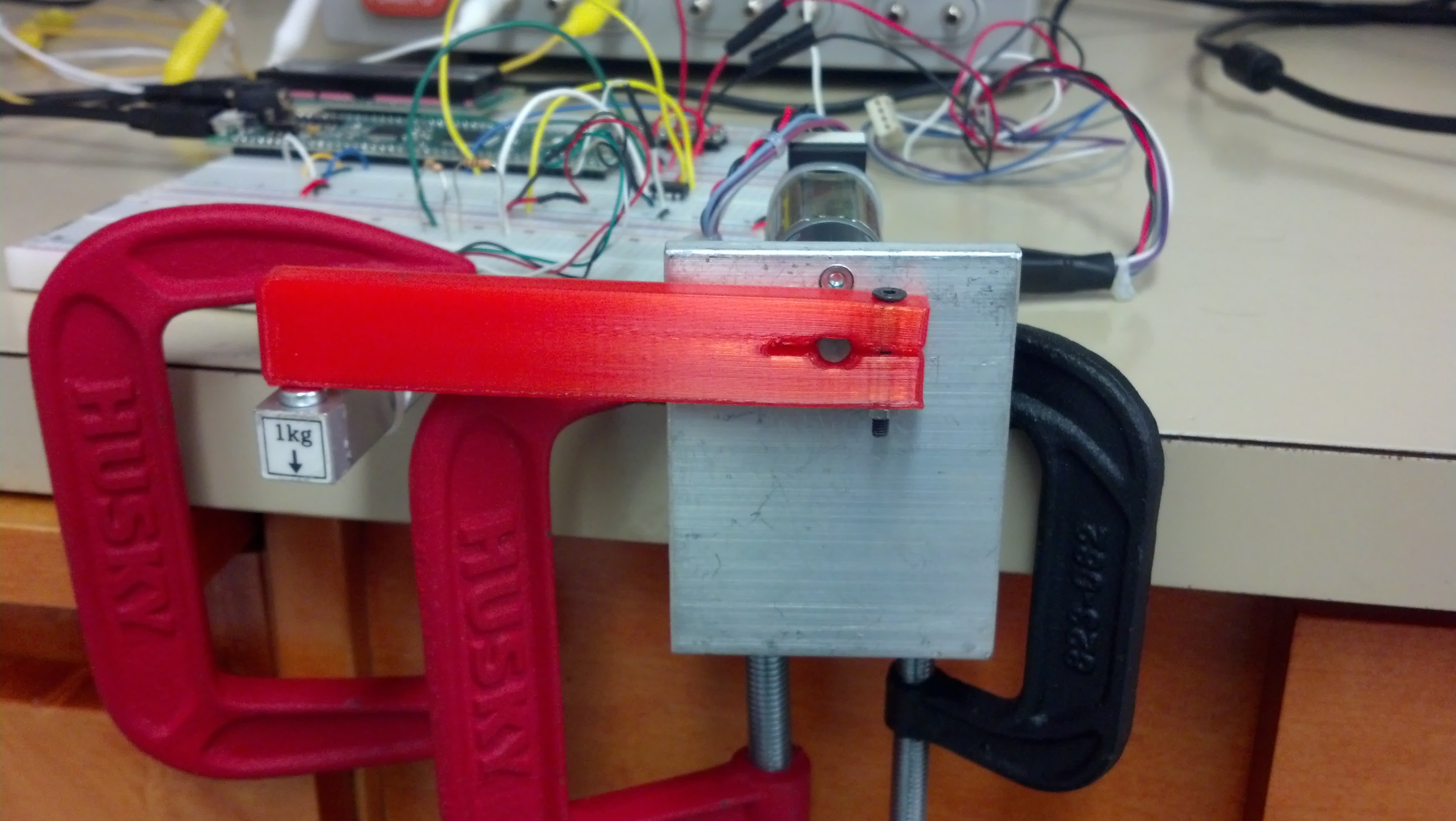
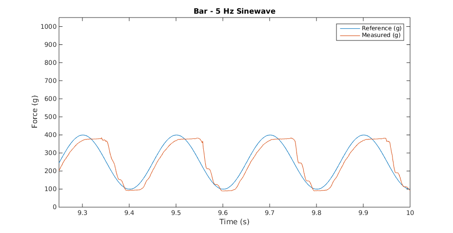
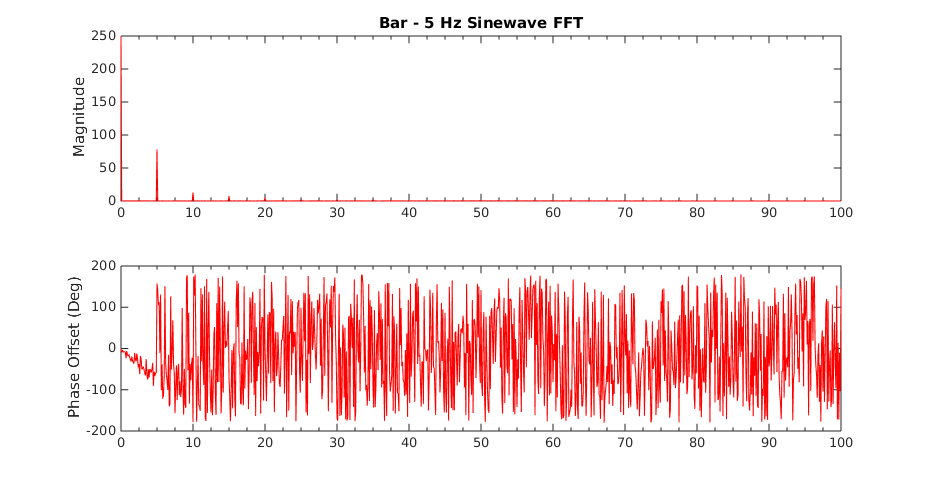
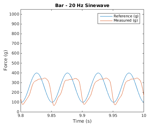
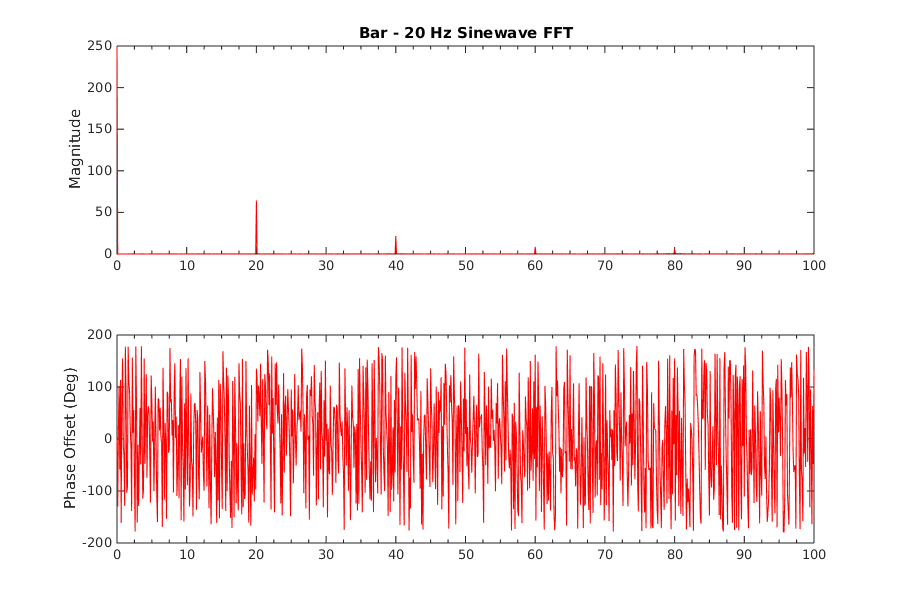
To characterize the behavior of a closed-loop system that has been changed to utilize the BioTac, the system was first tested with a simple straight bar as shown in the image. The system was tested by using sinusoidal force waveforms varying in frequency from 1 Hz to 20 Hz and varying between 100 g (0.98 N) and 400 g (3.92 N) of force for 10 seconds at a time. The results were recorded by the PIC and sent to the PC where they were analyzed using a fast Fourier transform to determine the relative magnitude and phase shift of the applied force as measured by the load cell compared to the reference waveform.
Once the system had been characterized using the bar, the bar was replaced by the BioTac and was put through the same tests. This data was recorded and analyzed in the same manner as for the bar.
Results
The following Bode plots demonstrate the results of the analysis of testing the closed-loop system with the bar and the BioTac.
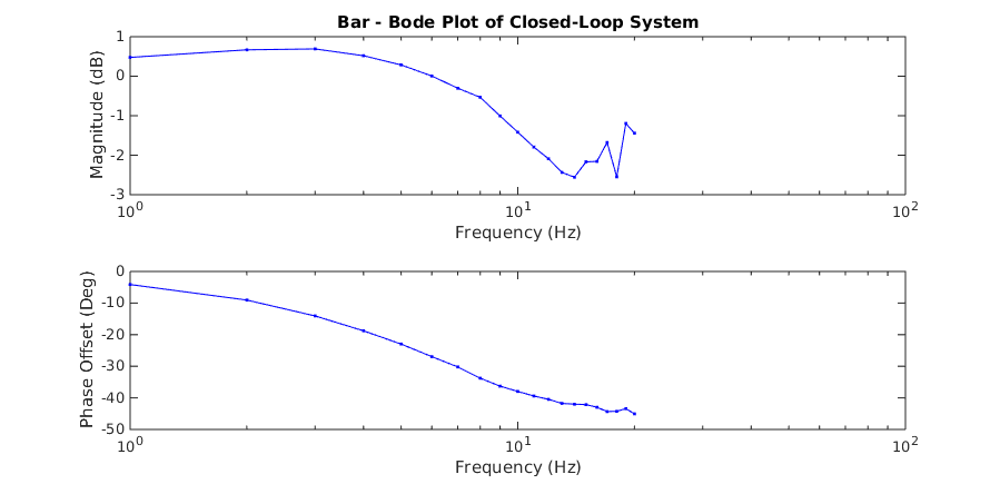
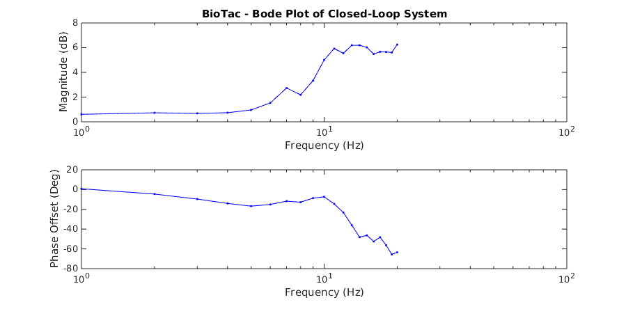
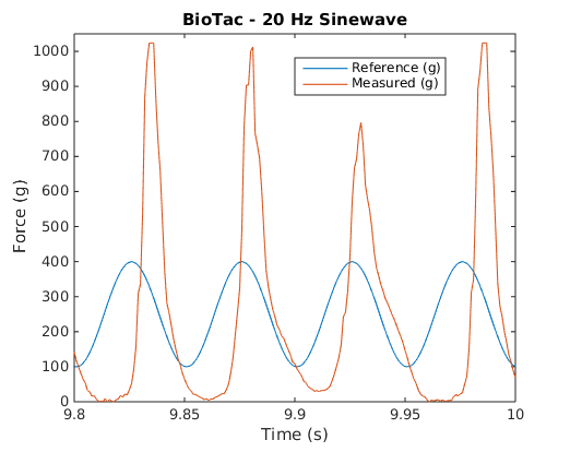
When the system is operating on the bar, it has a mostly linear response up to about 14 Hz. Beyond this point it starts to exhibit nonlinear behavior, most likely due to the motor nonlinearities beginning to affect the system. In contrast, the BioTac becomes quickly non-linear starting at about 6 Hz. This introduction of non-linearity is due to resonances building up within the fluid as it is subjected to regular sinusoidal force inputs. The following plots show some examples of recorded waveforms of the bar and their corresponding fast Fourier transforms at various frequencies.
| Bar Recorded Waveforms | Bar FFTs |
|---|---|
 |
 |
 |
 |
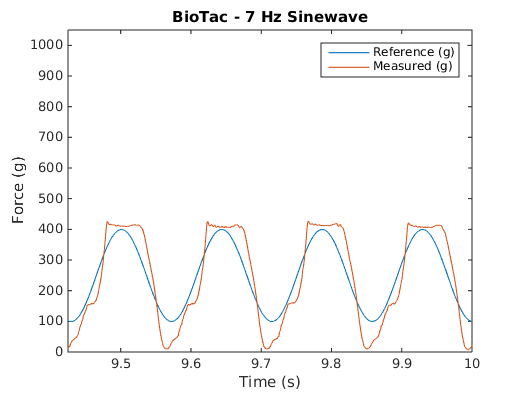
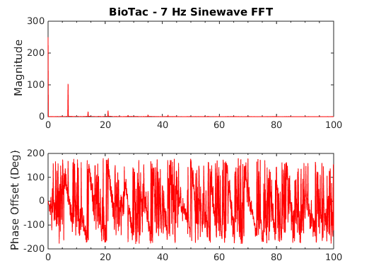
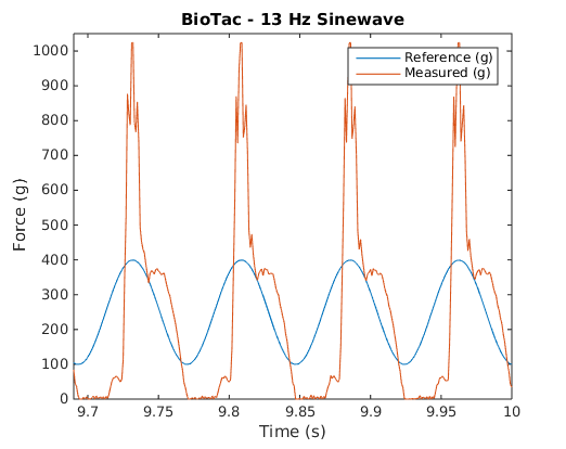
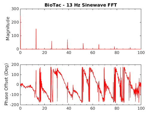
These plots show recorded waveforms and corresponding FFTs for the BioTac.
| BioTac Recorded Waveforms | BioTac FFTs |
|---|---|
 |
 |
 |
 |
 |
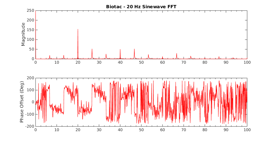 |
Notice the harmonics that appear in the BioTac plots but not in the bar. Also notice that these harmonics have higher and higher amplitudes relative to the reference frequency as well as the other harmonics.
Conclusions
The closed-loop system contains its own non-linearities, such as those inherent in the motor gearing as well as the effects of the integral term at higher frequencies. However, adding the BioTac to this system added a high degree of non-linearity. This makes sense given that the BioTac consists of a fluid-filled elastic membrane that can easily start to build up resonance. This project did not go as far as to accurately characterize the BioTac itself. However, it should be possible to modify the controller such that it can anticipate the BioTac’s behavior and help to mitigate any resonances it might build up in the fluid. Likely the feedforward term made it easier for the resonances to build up due to the way it aggressively tries to track the trajectory.
References
[1] C. H. Lin, J. A. Fishel and G. E. Loeb, “Extracting Point of Contact, Force and Torque in a Biomimetic Tactile Sensor with Deformable Skin”, SynTouch LLC, 2013
Source Code
The source code used in this project can be found here.